Differential Item Functioning with IRW Data

A DIF analysis needs two things: a response matrix, and a grouping variable whose order lines up with the rows of that matrix. The second one is the awkward part of the IRW workflow, because irw_long2resp() returns only id, item, and the response – person covariates are dropped, and some people may be dropped too. This article uses irw_covariates() to keep the two in step, then runs DIF with difR and calibrates items with irtoys.

library(irw)
library(difR)
library(irtoys)

The data

Many IRW tables carry person covariates in columns prefixed cov_, and irw_filter() will find them:

irw_filter(var = "cov_")
df <- irw_fetch("swmd_mokken")

Fetching needs Redivis credentials that this documentation build does not have, so the article builds a table with a known answer instead. Two groups of 400 people answer the same 10 items; items 3 and 7 are one logit harder for the focal group and the other eight behave identically. Sixty people, chosen at random, answered only the first three items – IRW tables are frequently ragged like this, and it matters below.

a <- rep(1.2, 10)
b_reference <- seq(-1.5, 1.5, length.out = 10)
b_focal <- b_reference
b_focal[c(3, 7)] <- b_focal[c(3, 7)] + 1

reference <- irw_simdata(n_id = 400, n_item = 10, model = "2PL",
                         a = a, b = b_reference, seed = 11)
focal <- irw_simdata(n_id = 400, n_item = 10, model = "2PL",
                     a = a, b = b_focal, seed = 12)
focal$id <- focal$id + 1000

reference$cov_group <- "reference"
focal$cov_group <- "focal"
df <- rbind(reference, focal)

set.seed(9)
quit_early <- sample(unique(df$id), 60)
df <- df[!(df$id %in% quit_early & df$item %in% 4:10), ]
head(df, 3)
#>   id item resp cov_group
#> 1  1    1    0 reference
#> 2  2    1    1 reference
#> 3  3    1    0 reference

Why alignment needs care

Pivot to wide and build the response matrix:

wide <- irw_long2resp(df, id_density_threshold = 0.5)
#> 60 ids removed (60 out of 800, 7.5%) due to response density below threshold (0.5).
#> To disable filtering, set `id_density_threshold = NULL`.
resp <- as.matrix(wide[, setdiff(names(wide), "id"), drop = FALSE])
rownames(resp) <- wide$id
dim(resp)
#> [1] 740  10

Two things happened. cov_group is gone, because irw_long2resp() keeps only the response columns. And the density filter dropped the 60 people who quit early, so the matrix has fewer rows than the long data has people:

length(unique(df$id))
#> [1] 800
nrow(wide)
#> [1] 740

That is what makes hand-alignment risky. Taking the covariate in its original order gives a vector of the wrong length:

naive <- df$cov_group[!duplicated(df$id)]
length(naive) == nrow(resp)
#> [1] FALSE

Had the filter dropped nobody, this would have produced a vector of the right length that was still wrong whenever the wide row order differed from first appearance – a silent error rather than a loud one.

irw_covariates() reduces the long data to one row per person and, given align, returns those rows in the order of the wide matrix:

people <- irw_covariates(df, align = wide)
head(people)
#>   id cov_group
#> 1  1 reference
#> 2  2 reference
#> 3  4 reference
#> 4  5 reference
#> 5  6 reference
#> 6  7 reference

identical(people$id, wide$id)
#> [1] TRUE
table(people$cov_group)
#> 
#>     focal reference 
#>       370       370

group <- people$cov_group

Logistic regression DIF

dif <- difLogistic(resp, group = group, focal.name = "focal")
colnames(resp)[dif$DIFitems]
#> [1] "item_1" "item_3" "item_7" "item_8" "item_9"

Statistical significance is easy to reach with hundreds of people per group, so read the effect sizes rather than the flags:

round(dif$deltaR2, 4)
#>  [1] 0.0150 0.0055 0.0574 0.0074 0.0003 0.0021 0.0591 0.0107 0.0180 0.0003

Items 3 and 7 – the two that were built to have DIF – have much the largest values. The other flagged items have effect sizes several times smaller, a reminder that a DIF flag at this sample size is not on its own evidence of a problem.

Mantel-Haenszel

A second method on the same inputs, as a cross-check. It flags the same items here, which is reassuring but not guaranteed in general:

mh <- difMH(resp, group = group, focal.name = "focal")
colnames(resp)[mh$DIFitems]
#> [1] "item_1" "item_3" "item_7" "item_8" "item_9"

Calibrating items with irtoys

irtoys wraps ltm and mirt behind one interface, which is convenient for quick estimates and plots:

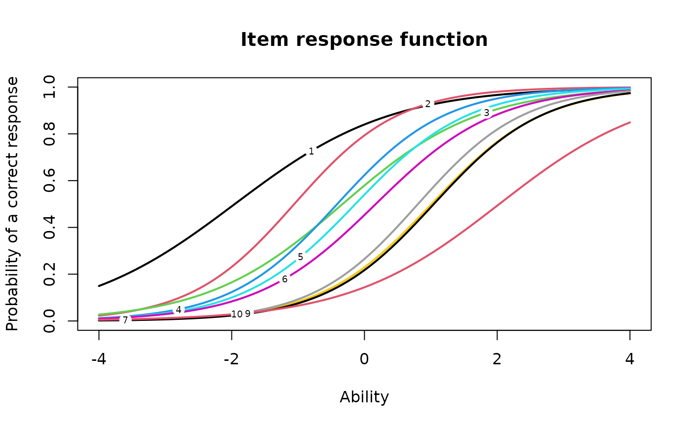
params <- est(resp, model = "2PL", engine = "ltm", nqp = 20)
head(round(params$est, 3))
#>         [,1]   [,2] [,3]
#> item_1 0.849 -1.953    0
#> item_2 1.274 -1.057    0
#> item_3 0.971 -0.330    0
#> item_4 1.232 -0.410    0
#> item_5 1.178 -0.136    0
#> item_6 1.104  0.170    0

The columns are discrimination, difficulty, and guessing. Calibrating the pooled sample recovers the generating difficulties reasonably well, except at the two DIF items, where pooling mixes two different difficulties:

data.frame(
  item = colnames(resp),
  b_reference = round(b_reference, 3),
  b_focal = round(b_focal, 3),
  b_pooled_estimate = round(params$est[, 2], 3)
)
#>            item b_reference b_focal b_pooled_estimate
#> item_1   item_1      -1.500  -1.500            -1.953
#> item_2   item_2      -1.167  -1.167            -1.057
#> item_3   item_3      -0.833   0.167            -0.330
#> item_4   item_4      -0.500  -0.500            -0.410
#> item_5   item_5      -0.167  -0.167            -0.136
#> item_6   item_6       0.167   0.167             0.170
#> item_7   item_7       0.500   1.500             1.011
#> item_8   item_8       0.833   0.833             0.807
#> item_9   item_9       1.167   1.167             1.046
#> item_10 item_10       1.500   1.500             2.032

plot(irf(params), co = NA, label = TRUE)