IRW tables arrive in long format with one row per response and the
columns id, item, and resp. Most
IRT packages want the opposite shape: a wide numeric matrix with one row
per person and one column per item. This article covers that handoff,
then fits the same data with three packages.
Getting the data
In normal use you fetch a table straight from the warehouse:
df <- irw_fetch("4thgrade_math_sirt")That call needs Redivis credentials, which this documentation build
does not have. So that these pages show real output, the rest of the
article runs on a simulated table with the same structure, via
irw_simdata():
df <- irw_simdata(n_id = 500, n_item = 12, model = "2PL", seed = 1)
str(df)
#> 'data.frame':    6000 obs. of  3 variables:
#>  $ id  : int  1 2 3 4 5 6 7 8 9 10 ...
#>  $ item: int  1 1 1 1 1 1 1 1 1 1 ...
#>  $ resp: int  1 0 1 1 1 0 0 1 1 1 ...
Checking responses before modelling
irw_check_resp() flags the two problems that most often
break an estimator: items where everyone gave the same answer, and
polytomous categories that are too thin to estimate.
checks <- irw_check_resp(df)
length(checks$single_category_items)
#> [1] 0
length(checks$sparse_category_items)
#> [1] 0
Long to wide
irw_long2resp() pivots to one row per person. It also
applies a default sparsity filter, dropping people who answered fewer
than 10% of items; pass id_density_threshold = NULL to keep
everyone.
wide <- irw_long2resp(df)
dim(wide)
#> [1] 500  13
wide[1:5, 1:5]
#>   id 1 2 3 4
#> 1  1 1 0 1 1
#> 2  2 0 0 0 0
#> 3  3 1 0 0 1
#> 4  4 1 1 1 1
#> 5  5 1 0 1 0
The result keeps id as a column, and its row and column
order is not sorted. IRT packages want just the item columns as a
matrix, so drop id and move it to the rownames:
resp <- as.matrix(wide[, setdiff(names(wide), "id"), drop = FALSE])
rownames(resp) <- wide$id
dim(resp)
#> [1] 500  12
That matrix is the input for everything below.
mirt
fit_2pl <- mirt(resp, 1, itemtype = "2PL", verbose = FALSE)
head(coef(fit_2pl, simplify = TRUE, IRTpars = TRUE)$items)
#>           a           b g u
#> 1 0.9916097 -1.17616700 0 1
#> 2 1.0404862  0.02815935 0 1
#> 3 0.7258002 -0.27193365 0 1
#> 4 1.0110873  0.14421691 0 1
#> 5 1.6778123 -0.34694119 0 1
#> 6 2.1691272  0.25794644 0 1
Person ability estimates come back in the row order of
resp, so they can be attached to the ids directly:
theta <- fscores(fit_2pl)
scores <- data.frame(id = rownames(resp), theta = as.numeric(theta))
head(scores)
#>   id      theta
#> 1  1 -0.2444948
#> 2  2 -1.0358841
#> 3  3 -1.0832246
#> 4  4  1.5453678
#> 5  5 -0.0254175
#> 6  6 -1.3443504
Comparing nested models is the usual way to justify the extra parameter:
fit_1pl <- mirt(resp, 1, itemtype = "Rasch", verbose = FALSE)
anova(fit_1pl, fit_2pl)
#>              AIC    SABIC       HQ      BIC    logLik      X2 df p
#> fit_1pl 7699.162 7712.689 7720.661 7753.952 -3836.581
#> fit_2pl 7594.016 7618.989 7633.707 7695.166 -3773.008 127.146 11 0
ltm
ltm takes a data frame rather than a matrix:
fit_rasch <- rasch(as.data.frame(resp))
head(coef(fit_rasch))
#>        Dffclt    Dscrmn
#> 1 -1.31724872 0.8504392
#> 2  0.03313202 0.8504392
#> 3 -0.23986786 0.8504392
#> 4  0.16408500 0.8504392
#> 5 -0.52860183 0.8504392
#> 6  0.43974219 0.8504392
psychotools
psychotools::raschmodel() is a lean
conditional-maximum-likelihood fit, handy when you want item
difficulties without a full IRT apparatus:
fit_pc <- raschmodel(resp)
head(itempar(fit_pc))
#>           1           2           3           4           5           6
#> -1.00852260  0.14050891 -0.09199266  0.25198548 -0.33781914  0.48650790
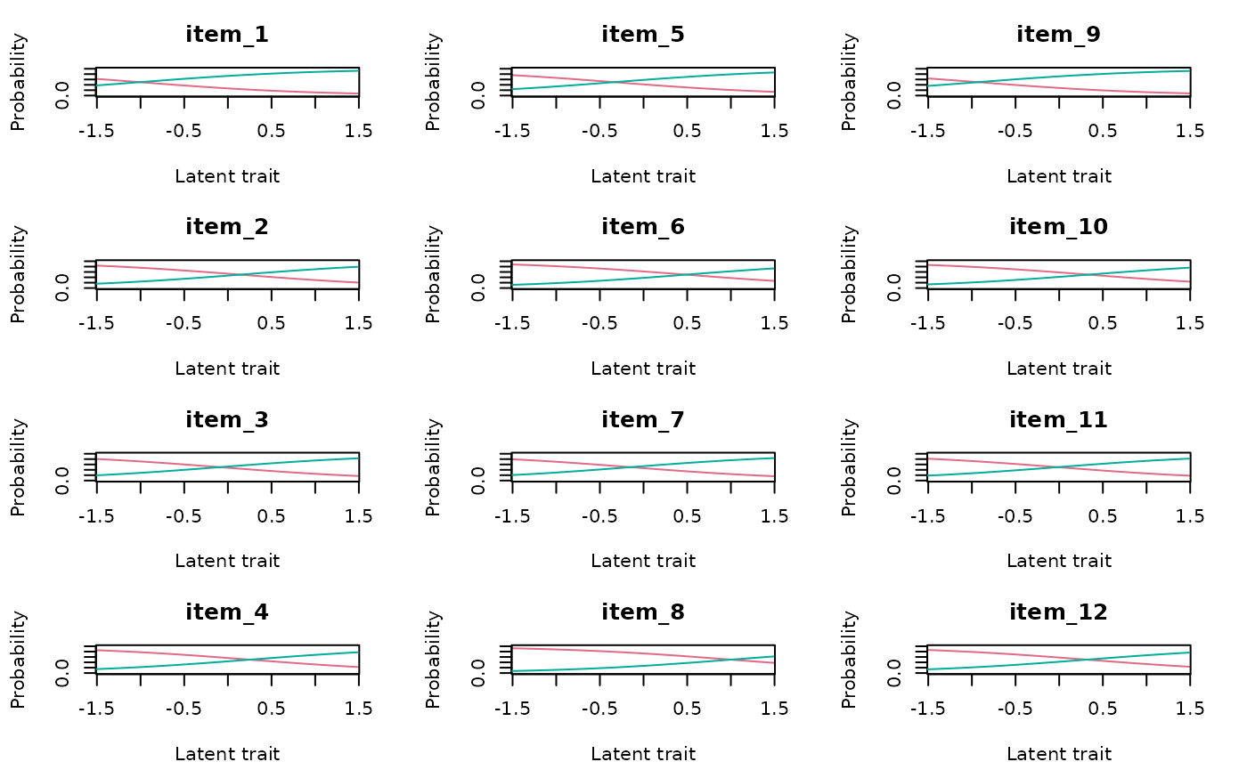
plot(fit_pc, type = "curves")